As the offshore wind industry gathers pace in US waters, we thought it would be a good time to illustrate the importance of simulating complex installation schedules to support efficient offshore planning.
It is common knowledge to the industry that US regulations mean that the installation of wind farms in US waters are restricted in their use of foreign vessels. In particular, the ‘Jones Act’ dictates that vessels transporting goods between two US locations need to be US built, flagged and owned. What this means is that construction strategies will need to consider non-US installation vessels staying offshore during construction and be fed by feeder barges from US ports and potentially from further afield.
This article shows how Mermaid® can be used to simulate a strategy whereby an installation vessel is bought over from Europe to the New Jersey waters and is then fed by three barges from two different supply ports (Paulsboro and New Bedford).
Each barge contains enough material to complete two installations. Each barge returns to port to reload and deliver back to the installation vessel four times, thereby installing twenty-four turbines. Mermaid is then used to analyse how long this process is likely to take depending on which month of the year the installation starts.
Model Set Up
The following sections shows how this operation can be set up using Mermaid and its easy to use graphical interface.
Map of Operations
The figures below show the map set up, detailing the turbine locations, three ports, transit routes and locations of metocean data.

Figure 1. Map of Model Set Up

Figure 2. Map of Wind Farm Zone
Vessels
Four vessels have been specified – one installation vessel and three identical feeder barges. The table below shows the station keeping and site arrival and departure weather limits that have been used. In this instance, we have just used a wind speed and wave height limit, other parameters could be used if required. The installation vessel has a speed of 15 knots and the feeder barges have a variable speed dependent on the wave height, as shown in Figure 3.
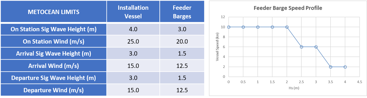
Table 1 / Figure 3. Table of Vessel Limits and Speed Profile
Operation Tasks
We have put together a relatively simply schedule to avoid over-complicating the analysis. It consists of three feeder barges servicing an installation vessel. Each feeder barge carries components for two installations and then returns to port to resupply and then returns offshore. When one barge has completed its load and installation cycle, the next barge meets the installation vessel at the next turbine, ensuring the installation vessel is not waiting needlessly. Two barges resupply from New Bedford and one from Paulsboro and the installation vessel mobs and demobs from European waters and transits to and from the site at the beginning and end of the schedule. The total ‘unweathered’ operation length is 57.5 days.
The installation tasks represent the weather windows required to unload from the barge and then three consecutive tasks of different durations, thresholds and repeats. Each individual task is ‘non-suspendable’, meaning that it can’t be interrupted. We do allow downtime in-between tasks, but the vessels must remain on site. Figure 4 gives a schematic of the tasks and Table 2 provides details of task durations and thresholds. Figure 5 shows how the schedule is shown in Mermaids uncluttered flow diagram, where the three coloured groups represent the tasks for each feeder barge.
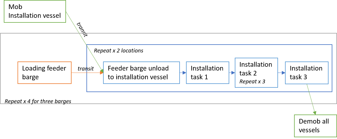
Figure 4. Schematic Flow Diagram of Operation Tasks
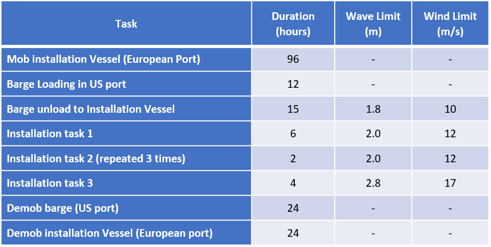
Table 2. Task Durations and Limits

Figure 5. Task Flow Diagram in Mermaid
Metocean Data
For this article we have used 10-years of modelled metocean time series data from close to the offshore site and for along the transatlantic route for the installation vessel. Ideally for a proper construction simulation we would use 20-30 years of data to gain a more accurate sense of the variability.
Mermaid has a useful inbuilt metocean statistics module which allows you to generate various weather occurrence and exceedance statistics for reference. For example, Figure 6 presents the monthly frequency distribution of significant wave height on site, showing that conditions are less than 2.0m for much of the time, indicating that wave height induced downtime should not be too severe.
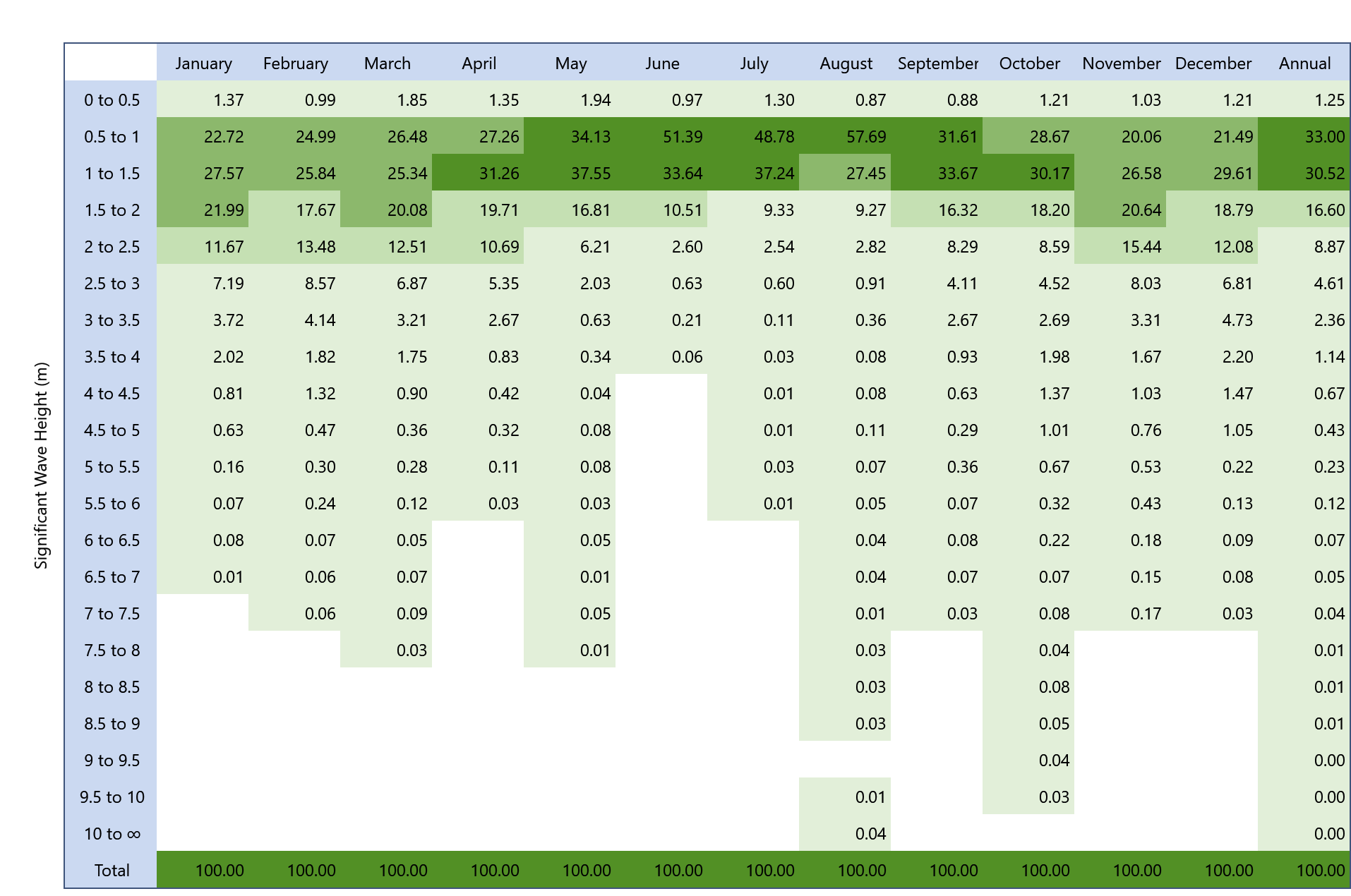
Figure 6 Monthly Frequency Distribution of Significant Wave Height at site
Results
We have tested the above schedule starting twice a month throughout the entire time series. This gives us 240 simulations of the operation, from which a wide range of duration and downtime statistics can be shown within Mermaid. Examples of which are shown below.
Figure 7 shows the monthly duration Box and Whisker plot, which shows the minimum, 25th, 50th, 75th percentile and maximum operation duration dependent on the start month. Figure 8 shows the operation duration exceedance statistics, this time aggregated for 3-month seasonal blocks. So, for example, in April the P50 (median) duration is 67 days and the P90 duration is 75 days (90% probability that duration will be up to 75 days).
Figure 8 also shows a quarterly Progress Burn Up Chart. This particular one shows the average time it takes to reach different percentage completion milestones of the entire installation. For example, when starting in November to January, on average it takes 45 days to reach the 50% completion mark and 65 days to reach the 75% mark. This diagnostic can be useful to see how a project is likely slow down or speed up due to weather as it progresses. The Progress Burn Up chart can also be used to study statistics on task milestones such as each individual installation, rather than percentage completion.
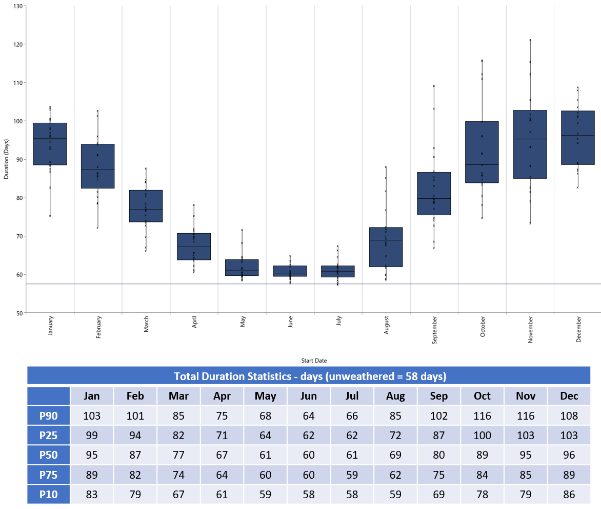
Figure 7. Box and Whisker Plot and Table showing Operation Duration Statistics
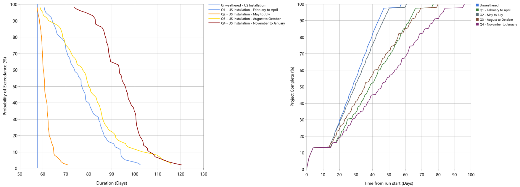
Figure 8. Quarterly Operation Duration Exceedence Statistics (left) and Progress Burn Up Chart (right).
From this selection of statistics, we can see an obvious seasonal trend that guides us as to when the best time to start operations would be. The downtime is clearly minimised if the operation starts between May and July with 2 to 3 days weather at the P50 level and 6-10 weather days at P90. The likelihood of downtime is at its greatest between October and January with 31 to 37-days at P50 and 45-58 weather days at P90.
The Progress Burn Up chart shows that the installation rate stays relatively consistent during each quarter, it typically takes 4 to 5 days to complete each 10% in the summer and 7 to 9 days in the winter.
Other charts and tables are available, such as tables of vessel usage and costs and project Gantt charts (figure 9).
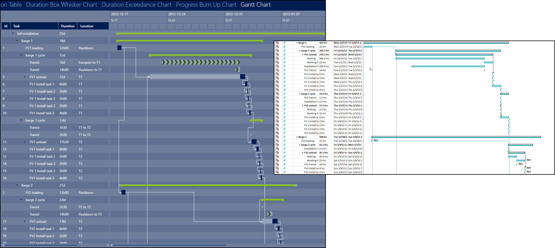
Figure 9 Gantt Chart of Schedule. in Mermaid format and when output to MS Project.
What Next?
The model built here can be very easily adapted to change various components to see if alternative strategies are more time and/or cost effective. Such changes could be:
- Use bigger barges so that more than 2 loads can be done at a time;
- Use more/less barges;
- Look at alternative supply ports;
- Use more than one installation vessel;
- Add further tasks to model to increase complexity and detail to the model.
Conclusions
We have shown how Mermaid can be used to build a realistic model of the installation of a wind farm in US waters in consideration of Jones Act regulations. The model has used multiple ports, both in the US and Europe, and a feeder vessel strategy to construct 24 turbines. Results show a clear seasonal trend where the optimum time to start this program is between May and July.
If you would like to know more about how Mermaid can be used to model and optimise your marine operations, then get in touch. We offer a free trial, complete with training.